Running ONTraC on a Xenium dataset
Download the data
The human breast cancer Xenium dataset originally published by Janesick, et al. is available at 10X genomics
For running this example, download the In Situ Sample 1, Replicate 1 (Xenium_FFPE_Human_Breast_Cancer_Rep1_outs.zip) and the Cell_Barcode_Type_Matrices.xlsx file
Data preparation
For this step, we will use the R package Giotto .
Read the Xenium data and create a Giotto object
library(Giotto)

expression_matrix <- get10Xmatrix("data_xenium/outs/cell_feature_matrix/",
                     gene_column_index = 2)

expression_matrix <- expression_matrix$`Gene Expression`

spatial_locs <- data.table::fread("data_xenium/outs/cells.csv.gz")
spatial_locs <- spatial_locs[, c("x_centroid", "y_centroid", "cell_id")]
colnames(spatial_locs) <- c("sdimx", "sdimy", "cell_ID")

instructions <- createGiottoInstructions(python_path = NULL,
                                       save_plot = TRUE,
                                       show_plot = FALSE,
                                       return_plot = FALSE,
                                       save_dir = "results_xenium")

xenium <- createGiottoObject(expression = expression_matrix,
                           spatial_locs = spatial_locs,
                           instructions = instructions)

cell_types <- cell_types$Cluster

xenium <- addCellMetadata(xenium,
                        new_metadata = cell_types)
Filter the cells with low counts
xenium <- filterGiotto(xenium,
                     feat_det_in_min_cells = 100,
                     min_det_feats_per_cell = 10)
Create the input table for ONTraC
metadata <- pDataDT(xenium)

coordinates <- getSpatialLocations(xenium,
                                 output = "data.table")

# create data table
dataset_table <- data.frame(Cell_ID = metadata$cell_ID,
                           Sample = rep("sample1_rep1", 163565),
                           Cell_Type = metadata$cell_types,
                           x = coordinates$sdimx,
                           y = coordinates$sdimy)


# subset region
write.table(dataset_table[dataset_table$x > 3000 & dataset_table$x < 4500  & dataset_table$y > 1000 & dataset_table$y < 2500, ],
            "dataset.csv", sep = ",",
            quote = FALSE, row.names = FALSE, col.names = TRUE)
Running ONTraC
If your default shell is not Bash, please adjust this code.
ONTraC will run on CPU if CUDA is not available.
conda activate ONTraC
ONTraC --meta-input dataset.csv \
--NN-dir selection/output_xenium/NN \
--GNN-dir selection/output_xenium/GNN \
--NT-dir selection/output_xenium/NT \
--device cpu --epochs 300 -s 42 --patience 100 \
--min-delta 0.001 --min-epochs 50 --lr 0.03 --hidden-feats 4 \
-k 4 --n-neighbors 50 --modularity-loss-weight 0.3 \
--regularization-loss-weight 0.1 --purity-loss-weight 300 \
--beta 0.03 > xenium_final.log
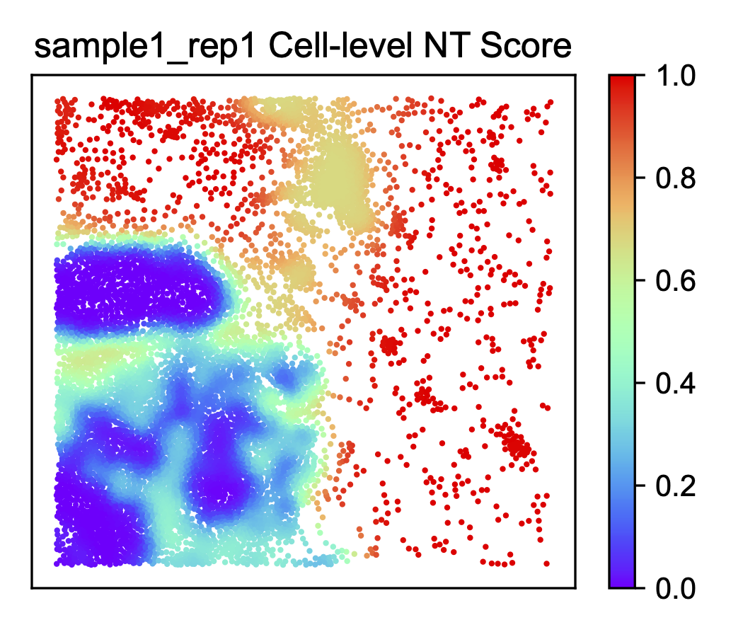
Results visualization
Please see the visualization tutorials for details.
Create all the plots with the ONTraC_analysis command.
ONTraC_analysis --meta-input dataset.csv \
--NN-dir selection/output_xenium/NN \
--GNN-dir selection/output_xenium/GNN \
--NT-dir selection/output_xenium/NT \
-o selection/analysis_xenium -l xenium_final.log